Consider a body on which there are several forces acting. We can isolate an element of unit area around a point P and measure the stresses \(\sigma\) and \(\tau\) along Cartesian axes as shown.
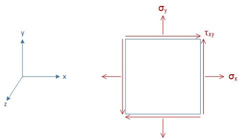
Stresses acting on an element in 2 dimensions
Notice that \(\sigma_x\) is acting parallel to the x-axis and \(\sigma_y\) is acting parallel to the y-axis.
Let us now cut another element around the same point P but at an angle \(\theta\) to the x-axis. The normal and shear stresses acting on the element will be different. Let the x prime axis be at an angle to the x axis.
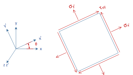
Stress on an element rotated by an angle to the x-axis
Therefore the stress we measure on an element around a point is dependent on its orientation. Since stress is a tensor, matrices are used to fully express the stress state in a material. For a 2D element, the matrix has the following form:
\(\large{\begin{bmatrix}
\sigma_{x} & \tau_{xy} \\
\tau_{xy} & \sigma_{y}
\end{bmatrix}}
\)
The following 3 stress transformation equations can be used for finding the stresses at other orientations than the one in which we are given.
The above equations can be used as simple ‘plug and chug’ in most cases of 2D stress transformations. In fact, these equations can be applied to any 2 dimensional tensor other than stress, including strain.
Mohr’s Circle
Christian Otto Mohr was a German Engineer who developed a way to graphically express the above stress transformation equations. His method makes it simple to understand stress variations on the element with changes in its orientation. His diagram is known as the Mohr’s Circle.
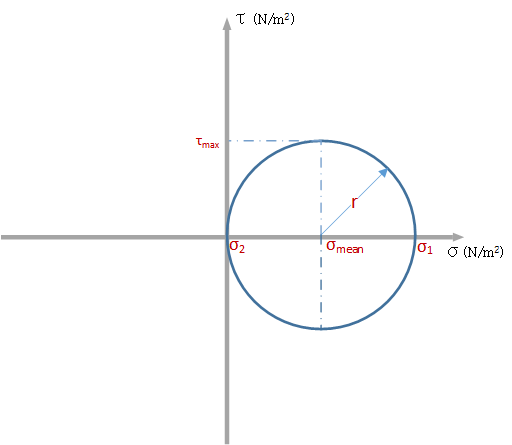
Mohr’s circle is used to represent the stress tensor graphically
The axes of the circle is made up by the normal \((\sigma)\) and shear stresses \((\tau)\). The cicle is drawn for 1 face of the element (normally the y face). The x face is found at a -90 degree rotation from the y face using the cartesian axes. But on the Mohr’s circle, rotations need to be doubled. This means that the x face is 180 degrees from the y face. Values for the x face is therefore found by making a 180 degree rotation from the point at which the stress for the y face is.
The circle itself is drawn by making use of 2 quantities, the average stress \((\sigma_{avg})\) and the radius \((R)\). Once the circle has been drawn, it becomes possible to extract additional information such as the principle stresses and the location of the principle axes from the plot.
Principal Stresses
Since the stress values vary depending on the angle \(\theta\), there is a special orientation at which the normal stresses \(\sigma\) will be maximum and minimum. These are known as the principal stresses. They are denoted by \(\sigma_1\) and \(\sigma_2\) with \(\sigma_1\) having the highest value.
Principal Axes
There is a special orientation at which the normal stress is maximum while the shear stress is zero. These are called the principal axes and are denoted by 1 and 2.